The Likelihood Ratio: Unveiling the Statistical Strength of Forensic Evidence

In the world of forensic science, a DNA profile is not an open-and-shut case; it’s a complex piece of data that demands rigorous interpretation. Juries, attorneys, and investigators don’t just want to know if a suspect’s DNA “matches” the evidence—they need to understand the strength of that evidence. How much more likely are we to see this specific DNA profile if the suspect is the source, versus if some unknown person is the source? This is the fundamental question that the Likelihood Ratio (LR) answers. It is the cornerstone of modern forensic statistical interpretation, transforming a simple observation into a quantifiable measure of evidential weight. This article will dissect the foundational science of the LR, walk through its application in forensic DNA analysis, and explore its profound implications in the pursuit of justice.

The Foundational Science of the Likelihood Ratio

At its core, the Likelihood Ratio is a concept rooted in Bayesian statistics, a framework for updating our beliefs about a proposition as we acquire new evidence. The LR doesn’t tell us the probability that a suspect is guilty—that’s the ultimate question for the jury. Instead, it focuses exclusively on the evidence itself, providing a balanced, logical, and scientifically defensible way to assess its value.

Bayes’ Theorem and the Role of Evidence

To grasp the LR, we must first appreciate its relationship with Bayes’ Theorem. The theorem provides a mathematical formula for updating the probability of a hypothesis based on new evidence. In a legal context, this can be expressed as:

Posterior Odds = Likelihood Ratio x Prior Odds

Here, the Prior Odds represent the odds of a proposition (e.g., the suspect is the source of the DNA) before considering the forensic evidence. The Posterior Odds are the updated odds after considering the evidence. The critical link between them is the Likelihood Ratio. The LR is the multiplier that tells us how much the new evidence should shift our belief in the proposition. A forensic scientist’s job is to calculate this multiplier, not to comment on the prior or posterior odds, which involve case information beyond the scope of their scientific analysis.

The Two Competing Hypotheses

The LR operates by comparing the probability of the evidence under two mutually exclusive hypotheses. This structure ensures a balanced and fair evaluation. These hypotheses are typically framed from the perspectives of the prosecution and the defense:

• The Prosecution Hypothesis (H_p): This proposition asserts that the suspect is the source of the evidential DNA. For example, “The DNA recovered from the crime scene is from John Doe.”
• The Defense Hypothesis (H_d): This proposition posits an alternative source for the DNA. For example, “The DNA recovered from the crime scene is from an unknown, unrelated individual in the relevant population.”

The scientist then asks: What is the probability of observing this specific DNA evidence profile if the prosecution’s hypothesis is true? And what is the probability of observing it if the defense’s hypothesis is true?

The Likelihood Ratio Formula

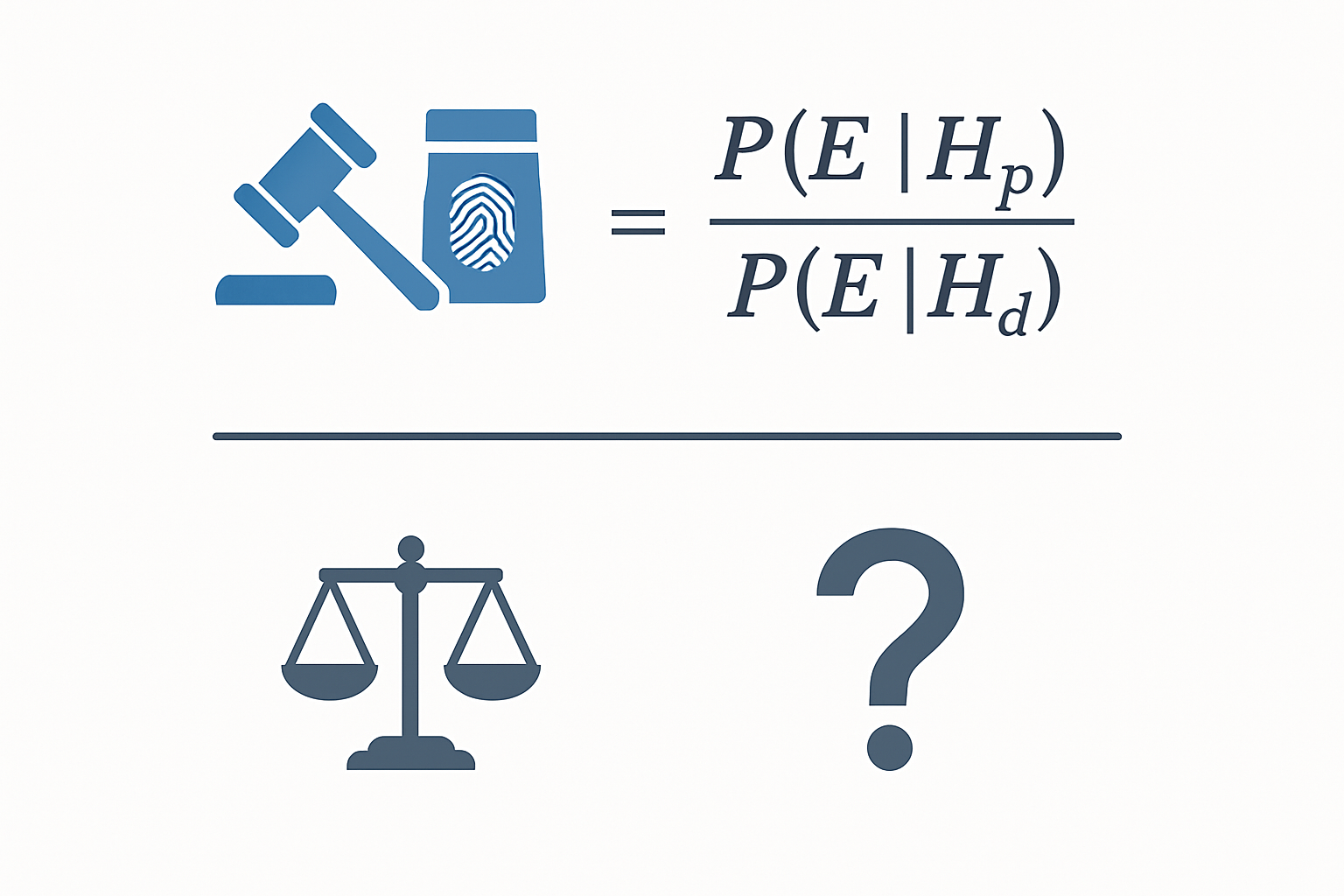
The Likelihood Ratio is the ratio of these two probabilities. The formula is elegantly simple but profoundly powerful:

LR = P(E|H_p) / P(E|H_d)

Where:

• E is the observed evidence (e.g., the DNA profile).
• P(E|H_p) is the probability of observing the evidence, given that the prosecution’s hypothesis is true.
• P(E|H_d) is the probability of observing the evidence, given that the defense’s hypothesis is true.

The resulting number is a direct measure of the strength of the evidence.

• An LR > 1 supports the prosecution’s hypothesis. For example, an LR of 1,000 means the evidence is 1,000 times more likely if the suspect is the source than if an unknown person is the source.
• An LR < 1 supports the defense’s hypothesis.
• An LR = 1 means the evidence is uninformative; it doesn’t support one hypothesis over the other.

The Core Forensic Process of the Likelihood Ratio in Detail

Applying the Likelihood Ratio to a real-world DNA sample is a multi-stage process that combines meticulous laboratory work with sophisticated statistical modeling. It moves far beyond a simple “match/no match” declaration to provide a nuanced weight of evidence.

Stage 1: Evidence Collection and DNA Profiling

The process begins at the crime scene. Forensic technicians collect biological material (e.g., blood, saliva, skin cells) from which DNA can be extracted. Back in the laboratory, this DNA is quantified, and specific regions are amplified using the Polymerase Chain Reaction (PCR). The focus is on Short Tandem Repeats (STRs)—short, repeating segments of DNA that vary greatly between individuals. The resulting DNA profile is visualized as an electropherogram, which shows peaks representing the different alleles (variants) at each STR locus (location). A reference profile is also generated from the suspect.

Stage 2: Formulating the Hypotheses

With the evidence profile (E) and the suspect’s reference profile in hand, the analyst formulates the pair of hypotheses.

• H_p (Prosecution): The DNA evidence came from the suspect.
• H_d (Defense): The DNA evidence came from an unknown, unrelated individual.

Let’s consider a simple, single-source sample from a crime scene and a suspect, “Mr. Smith.”

• H_p: The source of the crime scene DNA is Mr. Smith.
• H_d: The source of the crime scene DNA is an unknown, unrelated individual.

Stage 3: Calculating the Probabilities

This is the statistical heart of the process. The analyst calculates the probability of observing the evidence under each hypothesis.

• Calculating P(E|H_p) (The Numerator):This is often the more straightforward part. If the prosecution’s hypothesis is true (the suspect is the source), what is the probability of seeing the evidence profile? Assuming our lab techniques are perfect, if Mr. Smith is the source, we expect to see his DNA profile. Therefore, the probability of observing his profile, given he is the source, is essentially 1. In practice, we account for the small possibilities of error or mutation, but for a clean, single-source profile, this value is very close to 1.
• Calculating P(E|H_d) (The Denominator):This is the probability of seeing this evidence profile if an unknown, unrelated person is the source. To calculate this, we need to know how common or rare the specific alleles in the profile are. This is where population genetics comes in. Forensic laboratories use large, anonymous population databases that provide allele frequencies for different ethnic groups. The frequency of a complete multi-locus DNA profile is calculated by multiplying the frequencies of the individual genotypes at each locus, a principle derived from the Hardy-Weinberg equilibrium. This is often called the Random Match Probability (RMP). For example, if the genotype at one locus occurs in 1 in 100 people and at a second locus in 1 in 50 people, the combined profile frequency is 1 in 5,000 (100 x 50). With the 20+ STR loci used today, this probability becomes infinitesimally small.

Stage 4: Analysis & Interpretation

Once both probabilities are calculated, the LR is determined.

Let’s say for a given profile:

• P(E|H_p) = 1
• P(E|H_d) = 1 in 1 billion (or 10^-9)

The Likelihood Ratio would be:

LR = 1 / 10^-9 = 1,000,000,000

The scientist would then report this finding in a neutral, impartial manner. A typical statement might be:

“The DNA evidence is 1 billion times more likely to be observed if the suspect, Mr. Smith, is the source of the sample than if the source is an unknown, unrelated individual.” This statement is powerful, precise, and avoids the “prosecutor’s fallacy” of stating the probability of guilt. It correctly frames the result in terms of the evidence itself, leaving the ultimate conclusion to the court.

Advanced Applications & Modern Implications

The simple single-source example illustrates the core principle, but the true power of the Likelihood Ratio framework shines in more complex scenarios, which are increasingly common in forensic casework.

Advanced Applications: Probabilistic Genotyping

Modern forensic evidence often consists of complex DNA mixtures from multiple contributors or low-quality, degraded samples. In these cases, it’s impossible to cleanly separate one person’s profile from another. This is where probabilistic genotyping software (PGS) becomes essential. PGS uses complex computer algorithms and statistical models (like Markov Chain Monte Carlo) to consider thousands or millions of possible genotype combinations that could explain the observed mixture.

Instead of making a simple comparison, the software calculates an LR for a person of interest by comparing the probability of observing the mixed evidence if the suspect is a contributor versus if they are not. This approach allows analysts to interpret evidence that would have been deemed inconclusive just a decade ago, providing robust statistical weight to previously unusable data.

Case Study: The Likelihood Ratio in Practice

Consider a sexual assault case where a swab contains a mixture of DNA from the victim and an unknown male. A suspect is identified. The analyst uses probabilistic genotyping software to evaluate the evidence.

• Hypotheses:
  • H_p: The DNA mixture is from the victim and the suspect.
  • H_d: The DNA mixture is from the victim and an unknown, unrelated male.

The software runs simulations to determine how well the suspect’s DNA profile “fits” into the mixture compared to random profiles from the population. After analysis, the software might generate a Likelihood Ratio of 500,000. The expert testimony would be: “The mixed DNA profile is 500,000 times more likely if the sample originated from the victim and the suspect than if it originated from the victim and an unknown, unrelated male.” This provides the jury with a clear, quantitative measure of how strongly the DNA evidence links the suspect to the crime, even in a complex scenario.

Challenges, Controversies, and the Future

Despite its power, the LR is not without challenges. Its implementation requires sophisticated software, extensive training, and clear communication in the courtroom. Defense attorneys may challenge the underlying population databases, the assumptions of the software, or the formulation of the hypotheses. It is crucial that forensic scientists present the LR not as an infallible number but as a statistical estimate based on specific models and data.

The future of forensic statistics is undoubtedly tied to the continued refinement of probabilistic genotyping and the expanded use of the LR framework beyond DNA to other evidence types, like fingerprints and toolmarks. As our ability to generate data grows, so too must our statistical tools for interpreting it, ensuring that the evidence presented in court is not only present but also properly weighted and understood. The use of a Likelihood Ratio moves forensic science from a qualitative art to a quantitative science, a transition that is essential for the integrity of the criminal justice system.

Conclusion

The Likelihood Ratio is more than just a formula; it’s a logical framework for thinking about and communicating the value of evidence. By focusing on comparing competing, relevant propositions, it forces scientific experts to remain within their lane, presenting the court with what the evidence shows and nothing more. It avoids overstating conclusions and prevents the dangerous leap from a DNA match to an assumption of guilt. For students, practitioners, and legal professionals, a deep understanding of the LR is no longer optional—it is fundamental to the responsible application of forensic science. It provides the crucial, transparent, and defensible bridge between the laboratory bench and the witness stand.

FAQs: